42 format data labels excel 2016
How to Print Labels from Excel - Lifewire Select Mailings > Write & Insert Fields > Update Labels . Once you have the Excel spreadsheet and the Word document set up, you can merge the information and print your labels. Click Finish & Merge in the Finish group on the Mailings tab. Click Edit Individual Documents to preview how your printed labels will appear. Select All > OK . Prepare your Excel data source for a Word mail merge In your Excel data source that you'll use for a mailing list in a Word mail merge, make sure you format columns of numeric data correctly. Format a column with numbers, for example, to match a specific category such as currency. If you choose percentage as a category, be aware that the percentage format will multiply the cell value by 100.
Conditional formatting for chart axes - Microsoft Excel 2016 Chart Data Format Formula Interactive chart Macro Navigation Print Protection Review Search Settings Shape Shortcuts Style Tools. Outlook All Outlook. ... To change the format of the label on the Excel 2016 chart axis, do the following: 1. Right-click in the axis and choose Format Axis ...

Format data labels excel 2016
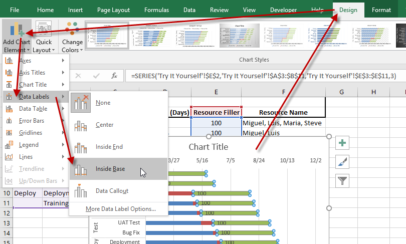
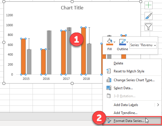
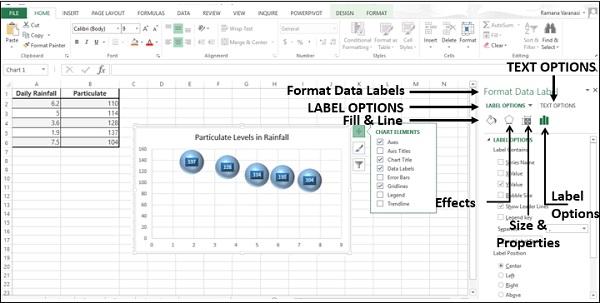
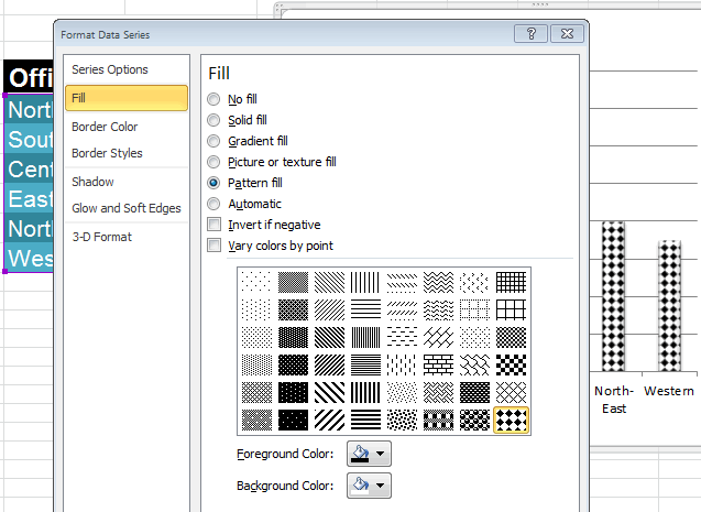
How to create Custom Data Labels in Excel Charts - Efficiency 365 Create the chart as usual. Add default data labels. Click on each unwanted label (using slow double click) and delete it. Select each item where you want the custom label one at a time. Press F2 to move focus to the Formula editing box. Type the equal to sign. Now click on the cell which contains the appropriate label. Change the format of data labels in a chart To get there, after adding your data labels, select the data label to format, and then click Chart Elements > Data Labels > More Options. To go to the appropriate area, click one of the four icons ( Fill & Line, Effects, Size & Properties ( Layout & Properties in Outlook or Word), or Label Options) shown here. How to Add Total Data Labels to the Excel Stacked Bar Chart Apr 03, 2013 · Step 4: Right click your new line chart and select “Add Data Labels” Step 5: Right click your new data labels and format them so that their label position is “Above”; also make the labels bold and increase the font size. Step 6: Right click the line, select “Format Data Series”; in the Line Color menu, select “No line”
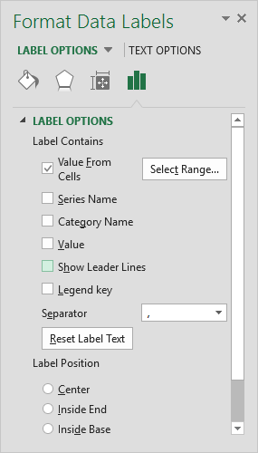
Format data labels excel 2016. Change the format of data labels in a chart To get there, after adding your data labels, select the data label to format, and then click Chart Elements > Data Labels > More Options. To go to the appropriate area, click one of the four icons ( Fill & Line, Effects, Size & Properties ( Layout & Properties in Outlook or Word), or Label Options) shown here. DataLabels object (Excel) | Microsoft Learn The following example sets the number format for data labels on series one on chart sheet one. With Charts(1).SeriesCollection(1) .HasDataLabels = True .DataLabels.NumberFormat = "##.##" End With Use DataLabels (index), where index is the data-label index number, to return a single DataLabel object. The following example sets the number format ... Excel 2016: "Value from Cells" box under Format Data Labels Missing 1. The screenshot about the issue. 2. The Office version screenshot via File > Account > Product Information. We will check whether the issue can be reproduced in a specific version. To protect your privacy, please help us mask email address like below: Thanks, Rena ----------------------- * Beware of scammers posting fake support numbers here. Excel 2016 Tutorial Formatting Data Labels Microsoft Training ... - YouTube FREE Course! Click: about Formatting Data Labels in Microsoft Excel at . A clip from Mastering Excel M...
Format Data Labels Vertically using Pareto in Excel 2016 Re: Format Data Labels Vertically using Pareto in Excel 2016. Try this: Right-click on one of the data labels > Format Data Labels > Size & Properties > Alignment > Text direction: Stacked. Register To Reply. 10-03-2017, 01:19 PM #3. 1gambit. Registered User. Format Data Labels in Excel- Instructions - TeachUcomp, Inc. To format data labels in Excel, choose the set of data labels to format. To do this, click the "Format" tab within the "Chart Tools" contextual tab in the Ribbon. Then select the data labels to format from the "Chart Elements" drop-down in the "Current Selection" button group. Excel charts: add title, customize chart axis, legend and data labels Click anywhere within your Excel chart, then click the Chart Elements button and check the Axis Titles box. If you want to display the title only for one axis, either horizontal or vertical, click the arrow next to Axis Titles and clear one of the boxes: Click the axis title box on the chart, and type the text. 5 Ways to Concatenate Data with a Line Break in Excel Sep 15, 2022 · The data appears to be all on one line still!”. Trust me, the line break characters are there. We need to format the cells to wrap text in order to see the results. Select any cells you want to format and right click and choose Format Cells from the options. You can also press Ctrl + 1 on your keyboard to open the Format Cells dialog box.
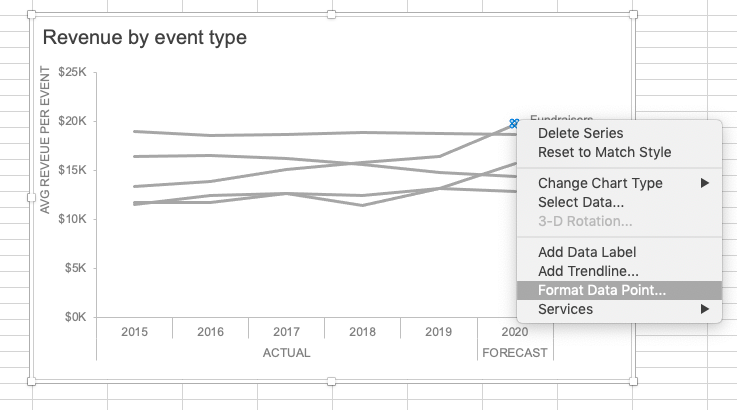
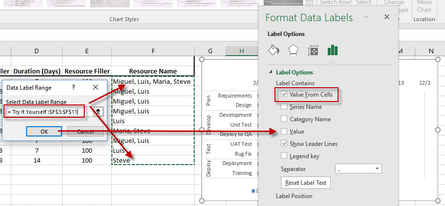
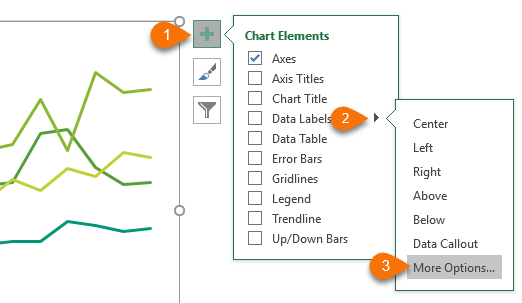
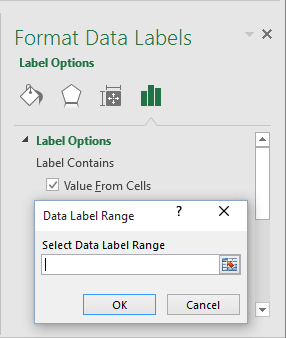
Excel 2016: How to Format Data and Cells - UniversalClass.com You can apply a number format to a cell by selecting the cell (s) that you want to format, right clicking, and selecting Format Cells and select the Number tab. You can also to the Home tab, go to the Number group, then click on the arrow in the bottom right corner. You will then see the Format Cells dialogue box. Add or remove data labels in a chart - support.microsoft.com Right-click the data series or data label to display more data for, and then click Format Data Labels. Click Label Options and under Label Contains , select the Values From Cells checkbox. When the Data Label Range dialog box appears, go back to the spreadsheet and select the range for which you want the cell values to display as data labels. How to rotate axis labels in chart in Excel? - ExtendOffice 1. Right click at the axis you want to rotate its labels, select Format Axis from the context menu. See screenshot: 2. In the Format Axis dialog, click Alignment tab and go to the Text Layout section to select the direction you need from the list box of Text direction. See screenshot: 3. Close the dialog, then you can see the axis labels are ... Edit titles or data labels in a chart - support.microsoft.com To edit the contents of a title, click the chart or axis title that you want to change. To edit the contents of a data label, click two times on the data label that you want to change. The first click selects the data labels for the whole data series, and the second click selects the individual data label. Click again to place the title or data ...
How to add live total labels to graphs and charts in Excel ...
How to Make Charts and Graphs in Excel | Smartsheet Jan 22, 2018 · To generate a chart or graph in Excel, you must first provide the program with the data you want to display. Follow the steps below to learn how to chart data in Excel 2016. Step 1: Enter Data into a Worksheet. Open Excel and select New Workbook. Enter the data you want to use to create a graph or chart.

Creating Pie Chart and Adding/Formatting Data Labels (Excel)
How to Print Labels from Excel - Lifewire Apr 05, 2022 · How to Print Labels From Excel . You can print mailing labels from Excel in a matter of minutes using the mail merge feature in Word. With neat columns and rows, sorting abilities, and data entry features, Excel might be the perfect application for entering and storing information like contact lists.Once you have created a detailed list, you can use it with other …

Chart data label alignment options greyed out in Excel 2016 ...
Excel 2016 VBA Display every nth Data Label on Chart I suggest to do following: Dim sData as Series For i = 1 to sData.Points.Count Step 4 sData.Points (i).ApplyDataLabels Next i. Note that if there is not value for the Point i in the series, the label seems not to be displayed. It took a while to find out why a label was not added to the chart.

Excel Custom Data Labels with Symbols that change Colors DYNAMICALLY with Data! - How To
excel - Change format of all data labels of a single series at once ... A quick way to solve this is to: Go to the chart and left mouse click on the 'data series' you want to edit. Click anywhere in formula bar above. Don't change anything. Click the 'tick icon' just to the left of the formula bar. Go straight back to the same data series and right mouse click, and choose add data labels.
/simplexct/BlogPic-h7046.jpg)
How to Create a Bar Chart With Labels Above Bars in Excel
How to Add Total Data Labels to the Excel Stacked Bar Chart Apr 03, 2013 · Step 4: Right click your new line chart and select “Add Data Labels” Step 5: Right click your new data labels and format them so that their label position is “Above”; also make the labels bold and increase the font size. Step 6: Right click the line, select “Format Data Series”; in the Line Color menu, select “No line”

Add or remove data labels in a chart
Change the format of data labels in a chart To get there, after adding your data labels, select the data label to format, and then click Chart Elements > Data Labels > More Options. To go to the appropriate area, click one of the four icons ( Fill & Line, Effects, Size & Properties ( Layout & Properties in Outlook or Word), or Label Options) shown here.
How to format Excel so that a data series is highlighted ...
How to create Custom Data Labels in Excel Charts - Efficiency 365 Create the chart as usual. Add default data labels. Click on each unwanted label (using slow double click) and delete it. Select each item where you want the custom label one at a time. Press F2 to move focus to the Formula editing box. Type the equal to sign. Now click on the cell which contains the appropriate label.

How to add total labels to stacked column chart in Excel?

Excel sunburst chart: Some labels missing - Stack Overflow

Apply Custom Data Labels to Charted Points - Peltier Tech

How to Place Labels Directly Through Your Line Graph in ...

PCWorld

Data Labels in Power BI - SPGuides
Custom Chart Labels Using Excel 2013 | MyExcelOnline
Excel 2016 Tutorial Formatting Data Labels Microsoft Training Lesson

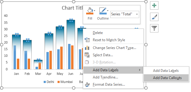
Add data labels and callouts to charts in Excel 365 ...

Apply Custom Data Labels to Charted Points - Peltier Tech
Excel 2016 Gantt Chart Modify Data Labels - Excel Dashboard ...
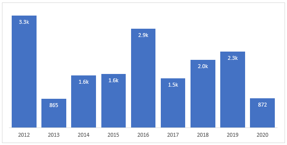
Format Chart Numbers as Thousands or Millions — Excel ...
Excel 2016 Gantt Chart Add Data Labels - Excel Dashboard ...

Change the format of data labels in a chart

Add data labels and callouts to charts in Excel 365 ...
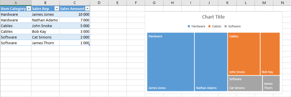
How to create a Tree Map chart in Excel 2016 | Sage Intelligence

Microsoft Excel Tutorials: Add Data Labels to a Pie Chart
Dynamically Label Excel Chart Series Lines • My Online ...
Format-Data-Series-for-Percentage-Chart-in-Excel - Automate Excel

Custom data labels in a chart

Visualizing high and low values across different scales in ...

Excel 2013 Tutorial Formatting Data Labels Microsoft Training Lesson 28.6

Custom data labels in a chart

Format Chart Numbers as Thousands or Millions — Excel ...
Creative Column Chart that Includes Totals in Excel
Excel Dashboards - Excel Charts

Change the format of data labels in a chart
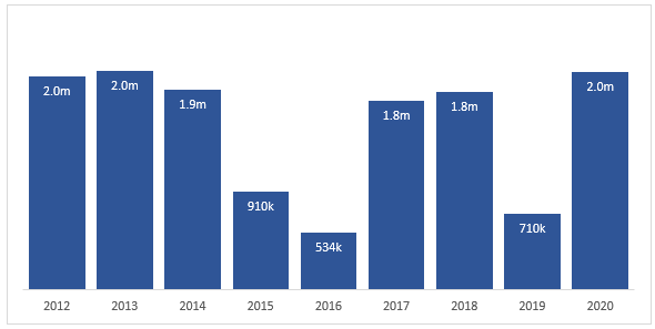
Format Chart Numbers as Thousands or Millions — Excel ...

How to Customize Your Excel Pivot Chart Data Labels - dummies

How to Change Excel Chart Data Labels to Custom Values?

Apply Custom Data Labels to Charted Points - Peltier Tech

How to format axis labels as thousands/millions in Excel?

How to Add Data Labels to an Excel 2010 Chart - dummies
Creating a chart with dynamic labels - Microsoft Excel 2016
Excel Charts: Tips, Tricks and Techniques
Post a Comment for "42 format data labels excel 2016"